An Evaluation of Measurement Decision Theory
Lawrence M. Rudner
Graduate Management Admission Council and LMP Associates

This research addresses the following questions:

1. Does measurement decision theory result in accurately classified examinees?
2. Are the different sequential testing procedures using decision theory as effective as maximum information item selection using item response theory?
3. How many items need to be administered to make accurate classifications? and
4. How many examinees are needed to satisfactorily calibrate measurement decision theory item parameters?

These questions are addressed using two sets of simulated data. In each case, predicted mastery states are compared against known, simulated true mastery states of examinees.

Examinees (simulees) were simulated by randomly drawing an ability value from normal N(0,1) and uniform (-2.5, 2.5) distributions and classifying each examinee based on this true score. Item responses were then simulated using Birnbaum=s (1968) three parameter IRT model. For each item and examinee, the examinee=s probability of a correct response is compared to a random number between 0 and 1. When the probability was greater than the random draw, the simulee was coded as responding correctly to the item. When the probability was less, the examinee was coded as responding incorrectly. Thus, as with real testing, individual simulees sometimes responding incorrectly to items they should have been able to answer correctly.

The items parameters were based on samples of items from the 1999 Colorado State Assessment Program fifth grade mathematics test (Colorado State Department of Education, 2000) and the 1996 National Assessment of Educational Progress State Eighth Grade Mathematics Assessment (Allen, Carlson, and Zelenak, 2000).

For each test, a calibration sample of 1000 examines and separate trial data sets were generated. The calibration sample was used to compute the measurement decision theory priors - the probabilities of a randomly chosen examinee being in each of the mastery states and the probabilities of a correct response to each item given the mastery state.

Key statistics for each simulated test are given in Table 1

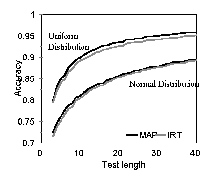
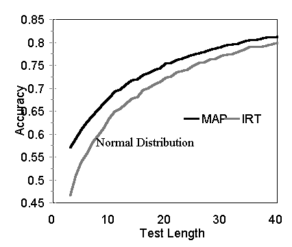
The simulated state-NAEP draws from a large number of items and a very reliable test. The cut scores correspond to the IRT theta levels that delineate state-NAEP=s Below Basic, Basic, Proficient and Advanced ability levels. The relatively small cell size for the Advanced level and the use of four mastery state classifications provide a good test for measurement decision theory.

The CSAP is a shorter test of lower reliability and the sample of items has mean difficulty (mean b) well below the mean examinee ability distribution. Classification categories are not reported for CSAP. The mastery/non-mastery cut score used in the study was arbitrarily selected to correspond to the 40^th percentile.

The accuracy of classifications using measurement decision theory relative to classifications using item response theory and the accuracy of sequential testing models relative to IRT computer adaptive testing were examined using these datasets. Accuracy was defined as the proportion of correct state classifications. To determine the correct state classification, the examinee=s true score was compared to the cut scores. To determine the observed classification, maximum a posterior (MAP) probabilities were used with the decision theory approaches and thetas estimated using the Newton-Raphson iteration procedure outlined in Baker (2001) were used with the IRT approach.

The reader should note that measurement decision theory approaches do not incorporate any information concerning how the data were generated, or any information concerning the distribution of ability within a category. The IRT baseline, on the other hand, was designed to provide a best case scenario for that model. The data fit the IRT model perfectly. Adaptive IRT testing used the items with the most information at the (usually unknown) true scores to optimally sequence the test items.

A key question is whether use of the model will result in accurate classification decisions. Accuracy was evaluated under varying test lengths, datasets, and underlying distributions. Test lengths were varied from 3 items to the size of the item pool. For each test length, 100 different tests were generated by randomly selecting items from the CSAP and NAEP datasets. For each test, 1,000 examinees and their item responses were simulated.

The results for select test sizes with the CSAP are shown in Table 2 and all CSAP values are plotted in Figure 1. There is virtually no difference between the accuracies of decision theory scoring and IRT scoring with either the uniform or normal underlying ability distributions. With the NAEP items, four classification categories, and normal examinee distributions, decision theory was consistently more accurate than IRT scoring (see Figure 2). With uniform distributions, IRT has a slight advantage until 25 items when the curves converge.

Figure 1: Accuracy of decision theory (MAP), and IRT scoring as a function of test length and ability distribution for simulated tests based on CSAP.

Figure 2: Accuracy of decision theory (MAP), and IRT scoring as a function of test length for simulated tests based on state-NAEP.

For this analysis, data sets of 10,000 normally distributed N(0,1) examinees and their responses to the CSAP and state-NAEP items were generated. Using these common datasets, items were selected and mastery states were predicted using three sequential testing approaches (minimum cost, information gain, and maximum discrimination) and the baseline IRT approach.

Under the IRT approach, the items with the maximum information at the examinee=s true score were selected without replacement. Thus, the procedure was optimized for IRT.

As shown in Table 3, the minimum cost and information gain decision theory approaches consistently out-performed the IRT approach in terms of classification accuracy. The fact that the classification accuracies for these two decision theory methods are almost identical implies that they tend to select the same items. Optimized to make fine distinctions across the ability scale, the IRT approach is less effective if one is interested in making coarser mastery classifications. The simple maximum discrimination approach was not as effective as the others, but was reasonably accurate.

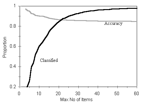
After each item was administered above, Wald=s SPRT was applied to determine whether there was enough information to make a decision and terminate testing. Power and error rate where set to α=β= .05. Table 4 shows the proportion of examinees for which a classification decision could be made, the percent of those examinees that were correctly classified, and the mean number of administered items as a function of maximum test length using items from state-NAEP. With an upper limit of only 15 items, for example, some 75% of the examinees were classified into one of the 4 NAEP score categories. A classification decision could not be made for the other 25%. Eighty-eight percent of those examinees were classified correctly into one of the 4 state-NAEP categories and they required an average of 9.1 items. SPRT was able to quickly classify examinees at the tails of this data with an underlying normal distribution.

The proportions classified and the corresponding accuracy as a function of the maximum number of items administered are shown in Figure 3. The proportion classified curve begins to level off after about a test size limit of 30 items. Accuracy is fairly uniform after a test size limit of about 10 or 15 items.

Figure 3: Proportion of examinees classified and the accuracy of those classifications as a function of the maximum number of administered items (state-NAEP items, four latent states, sequential testing using information gain, sequential decisions using SPRT).

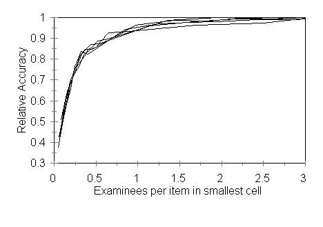
Another key question for any measurement model is the sample size needed to obtain satisfactory priors. With item response theory, the minimum acceptable calibration size is some 1000 examinees, which severely limits applications of the model.

The priors for the measurement decision theory model are the proportions of examinees in the population in each mastery state, P(m_k), and the probabilities of responding correctly (and consequently the probabilities of responding incorrectly) given each mastery state, P(z_i=1|m_k). These priors will usually be determined by piloting items with a calibration sample.

To determine the necessary number of calibration examinees, examinee classification accuracy as a function of calibration sample size and test size was assessed. Samples sizes of [20,30,40,50,60,70,80,90,100,200,300,400,500,600,700,800,900,1000] and test sizes of [5,10,15,20,25,30,35,40,45] were examined using state-NAEP and CSAP items. Under each condition, 100 tests were created by randomly selecting the appropriate number of items from the selected item pool. These tests were then each administered to 1000 simulees and the accuracy of the classification decision using MAP was determined.

Classification accuracy is usually best for tests calibrated on larger samples. In order to place the observed accuracies on a common scale, the accuracy of each sample size condition was divided by the accuracy of the corresponding 1000 calibration examinee condition to form a relative accuracy scale.

Accuracy of the priors is also limited by the size of the smallest cell. For the CSAP, this was always the non-masters (approximately 40% of the calibration sample). For NAEP, this was the Advanced category (approximately 17%). Variations due to cell size were controlled by dividing the number of calibration examinees in the smallest cell by the number of items on the simulated test. Thus, relative accuracy as a function of the number of calibration examinees per item in the smallest cell was used to help evaluate the needed calibration sample size.

Table 5 shows the results for 100 random 30 item tests using state-NAEP items. The data under the different test size conditions using state-NAEP items are quite similar and plotted in Figure 4. In Figure 4, the x-axis is truncated at 3 subjects per item. Beyond that value, the curves are flat. The results using CSAP were virtually identical. One can see from Figure 4 that relative accuracy levels off as the number of calibration examinees in the smallest cell approximates a little more than the test size. Thus, a random sample of only 25 to 40 examinees per cell would be needed to calibrate a 25 item test.

Figure 4: Accuracy of tests formed from state-NAEP items relative to tests calibrated with 1000 examinees as a function of the number of calibration examinees per item in the smallest cell.